Prologue
This article continues on the themes covered by the last two (here and here) relating to factorization and the primitive root modulo of a prime number. Early in ones education one learns the divisibility tests for the first few primes: 2, 3, and 5. Of these divisibility by 2 and 5 is trivial. Divisibility by 3 is also easily achieved: e.g. Is 771 divisible by 3?  . We see that the successive addition of digits reduces the original number to 6 which is divisible by 3; hence, the original number is divisible by 3. Of course, division by 3 is not a big deal; yet, for big numbers this is an easy method for mentally determining divisibility.
Beyond these three simple cases, in our school days we determined the divisibility by other primes using brute force — by dividing the test number by the given prime. When we reached college, a gentleman of great mathematical ability asked us if we could think of a generalization of the divisibility test for 3 for other primes. Seeing that we were unable to do so, he proceeded to tell us of such a method. He then mentioned that he had learned this via Suryanarayana of Vishakhapatnam who possessed enormous mathematical knowledge and capacity. Suryanarayana had further informed him that it was a folk Hindu method that was known in South India. Shortly thereafter, we saw the same method with some tricks for quick implementation in the pre-computer age described by the late Śaṃkarācarya Bhāratī Kṛṣṇa Tīrtha-jī (hereinafter SBKT) of the Govardhana pīṭha in his curious mathematical work with 16 foundational sūtra-s. He called the method veṣṭana, which he rendered in English as osculation, and presented it as an example of his sūtra: “ekādhikeṇa pūrveṇa |”
The Hindu divisibility test
The procedure goes thus:
1) Let  be a prime other than 2, 3, 5 for which divisibility is already accounted for. Let the test number be
  which is written as
  .
.
2) Find the first number  , i.e. the first multiple of which is of the form
  . Thus, this number will necessarily be of the form
  , where
  . That is how it relates to SBKT’s “ekādhikeṇa pūrveṇa |”
3) This  is termed the veṣṭaka or ‘osculator’ for the procedure. We then compute
  .
.
4) We again write  and repeat this procedure:
  .
.
5) If divides then this procedure terminates in a small and easily recognized multiple of . Any further application of the above procedure on that number yields the same number.
Let us illustrate it with an example: Is  divisible by
  ?
?
For ,  . Now we use the osculator
  for applying the above procedure.
We get 
We reach 19 indicating that 3249 is divisible by 19. Applying the above procedure to 19 yields 19 again. Indicating that it is a terminal number of the process. In a practical application from the pre-computer age we don’t have to go all the way: we could stop for e.g. at 38, which we recognize as a multiple of 19. Further, for bigger numbers SBKT gives certain tricks which would be useful in such pre-computer applications.
What if a number is not divisible by ? As an example consider the case: Is  divisible by 19? Of course, in this case the answer is quite obvious; nevertheless, it allows us to illustrate what happens if we apply the above procedure on it. We get the following sequence of
 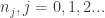 :
:

We observe that, unlike the divisible which converges to a single number, the non-divisible after the first 2 terms enters a repeating cycle of 18 terms. Again, for practical purposes if one just wanted to test divisibility one obtains the answer much earlier.
The basic divisibility graphs
We can do this divisibility procedure for several successive , say for all  and , and the illustrate the conglomerate results as an ordered graph (Figure 1). The graph’s nodes are the numbers
  obtained while applying the above divisibility procedure until we hit a cycle or converge. The edges indicate which number leads to which, with the relative thickness indicating the frequency with which they occur for this range of (scaled by hyperbolic arcsine).
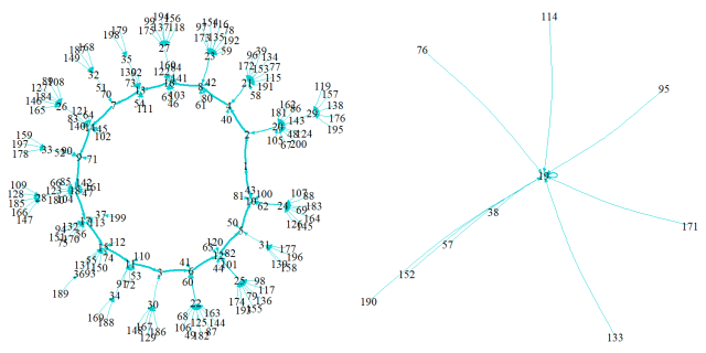 Figure 1
One also notices that all in this range, which are divisible by 19, directly converge to it. The remaining numbers converge directly or indirectly by different paths to a central directed ring  with components
  . These are the same as the terms of the cycle obtained in the above example. One also notices that in this example the ring size
  , i.e. number of terms in the ring, corresponds to cycle length of the decimal expansion of
  or
or  when
when  for the first time. This
  , in this case 18, is known as the multiplicative order of
  , which was shown by Carl Gauss to correspond to the cycle of the decimal expansion of
  . The terms of this ring includes all the number from
  . Thus, it is also obvious that the sum of the terms of in ring is divisible by :
To further explore these patterns, we next consider the case of  and plot the same for graph for in Figure 2.
 Figure 2
We observe that all divisible by 13 in this range converge to 3 terminal nodes: 13, 26 and 39. The remaining converge directly or indirectly to one of 6 rings with 6 terms each. i.e.  . Here again we notice that the size of these rings is the same as the multiplicative order of
  (
( when
when  for the first time), which is cycle length of the decimal expansion of of
  . Further, together the 6 rings include all numbers from 1..38 barring 13 and 26 which are divisible by 13. It is easy to see that
  is divisible by 13. However, we also notice that the sum of the terms of each of the six rings is also divisible by 13:
We next consider the case of  and (Figure 3).
 Figure 3
In this graph the numbers divisible by 7 converge to 2 endpoints either 7 itself or 49 (when they are multiples of 49). All the remaining numbers directly or indirectly converge to a large ring with 42 terms, which includes all numbers from 1..48 except for 7, 14, 21, 28, 35, 42. Thus, it is easy to see that the sum of the terms of this ring will be divisible by 7. Further, the multiplicative order of  is 6. Thus, the number of terms in the ring is multiple of that
  .
.
To sum up, we may note the following features of these divisibility graphs:
1) The residue system of for base 10 (till  for
for  produces 1 as the residue for the first time, i.e. till is equal to the multiplicative order) is: 10, 5, 12, 6, 3, 11, 15, 17, 18, 9, 14, 7, 13, 16, 8, 4, 2, 1. The base 10 residue system for is: 10, 9, 12, 3, 4, 1. The base 10 residue system of is: 3, 2, 6, 4, 5, 1. We observe that the penultimate residue in each case is what SBKT calls the “osculator” used in the divisibility test.
2) Looking the graphs, it becomes clear that the non-divisible converge to one or more directed rings, the sizes of which are either the multiplicative order  for base 10 or a multiple of . A number
  is a primitive root of if the residue system of
  contains all numbers from
  . If 10 is not a primitive root of the , the divisibility by which we are testing, then we will necessarily have multiple rings. If 10 is a primitive root of we can in some cases get a single ring with its terms being all numbers from (e.g. 19). Alternatively, we can get a large single ring whose size can be some multiple of the multiplicative order (e.g. ) or multiple rings whose sizes are different multiples of the multiplicative order (e.g.
  ).
).
 Figure 4. Divisibility graph for
3) The terms included in all the rings of convergence taken together for a given range from  , where is the penultimate residue of the system and the osculator. Of course, all numbers divisible by in this range are excluded from the rings as they are nodes of separate components of the graph that converge to single root, an integer divisible by . Thus, for , the osculator is
  . So, the integers covered in the rings would be from 1 to 38, with 13 and 26 not being in the rings. For , the osculator
  ; hence, the ring would cover the integers from 1 to 48, with 7, 14, 21, 28, 35, 42 being excluded. When , the osculator is
  . Thus, the rings will extend from 1 to 118, with 17, 34, 51, 68, 85, 102 being excluded.
4) From the above it is obvious that the sum of the numbers in all the rings taken together would be divisible by . The less obvious feature is that the sum of the numbers in each individual ring of the convergence graph is also divisible by . Thus, the numbers are placed in each ring in such a way that two constraints are simultaneously met, namely: 1)that of divisibility of the sum of the numbers in each ring by and 2) that of each ring size being a multiple of the base 10 multiplicative order modulo the given . In the case of placing the numbers in 6 separate rings can satisfy the above constraints for each ring. In the case of placing them in 3 separate rings can satisfy them, while in the case of they need to be in a single large ring to meet the constraints.
5) An obvious but structurally distinctive feature of the divisibility graph is that 1 can never be reached directly from any unless it is a member of the ring to which 1 belongs. From the procedure it is clear that it can be reached only from 10. 10 is the first number in the base 10 residue system for any  and will necessarily be part of the ring. Further, in whichever ring 1 occurs, by the nature of the procedure, it would always lead next to the osculator as the next node in the ring. always comes just before it in the residue system for base 10 (e.g. for 13: 10, 9, 12, 3, 4, 1): thus
  is fixed a motif in the divisibility ring reverse order of their occurrence in the residue system. The longest path of the divisibility graph ending in a ring always passes through this (However, there could be graphs with multiple equally long paths passing through other ring nodes in certain cases like ).
One wonders is an encryption system along the lines of the Diffie-Hellman-Merkle mechanism can be made using these divisibility graphs.
The reduced divisibility graphs
The above-described graphs were based on the simple divisibility method found in folk Hindu mathematics and SBKT’s mathematical exposition. However, for practical purposes SBKT gives an additional step, which he terms the “casting out of the primes”. This goes thus: We again write the test number as . We then obtain  , where is the osculator as above. Thus, we first reduce
  to its residue modulo the , the divisibility by which we are testing, before adding it to
  to arrive at
  .
.
As a numerical example let us consider testing the divisibility of 99 by 7. The osculator for 7 is . Thus  . We now take
  and use it in place of 45. Thus, we get
  which allows us to decide on the matter of divisibility right away. However, we could continue the procedure to convergence, as we did above, in order to compute the convergence graphs for different . In this case we observe the following:
1) If 10 is a primitive root of then we get a bipartite graph: One component derived from all the non-divisible has a central ring, which has as its terms all numbers from . The other component is a tree graph converging to which includes all the divisible by . Examples of this are the graphs for or
 Figure 5. The convergence graph for
 Figure 6. The convergence graph for
2) If 10 is not a primitive root of then we get a multipartite graph. One component, as above, is a tree graph converging on and includes all the divisible by . The remaining components have central rings whose size is the multiplicative order of  . The number of these ring components is
  . Here again, the sum of the numbers in each ring is divisible by . Together they include all integers from . Examples of this are the graphs for and
  .
.
 Figure 7. The convergence graph for . Here
  for base 10; thus we get
  components with central rings.
 Figure 8. The convergence graph for . Here
  for base 10; thus we get
  components with central rings.
In these graphs too the longest path terminating in a ring passes through the osculator , which is reached from 1 on the ring. Here again, 1 is reached from 10, the first residue of the residue system for base for all primes . However, given that  , for , 1 is reached from 3 in the ring. In conclusion, this version of the divisibility graph makes apparent the close relationship it has to the period of the decimal form of the fraction , which we considered in the previous article.

 Figure 1
 Figure 2
 Figure 3
 Figure 4. Divisibility graph for
  Figure 5. The convergence graph for
  Figure 6. The convergence graph for
  Figure 7. The convergence graph for
  Figure 8. The convergence graph for